
Learning from Projections
There we are. Welcome to this final part of a four-part series on learning from 3D data. After racking our brains to understand deep learning techniques in various 3D representations (point clouds, voxel grids, graphs and meshes), in this last episode we dial it back a notch, more precisely from three to two dimensions.
Why (not) to project
As always, the first question is, why should we want to do this?. Before we can answer this question, let’s first define what is meant by projection in this context1. In general, a projection is a mapping transforming something to something else. For geometric settings, i.e. when talking about mappings from one dimension to another, this is often referred to as projecting data from one representation to another. Depending on your background, you might think about dimensionality reduction techniques like PCA, projecting the data from a high to a lower dimensional space, neural networks, projecting (relatively) low dimensional inputs like images into higher dimensional feature space or photography, projecting our three dimensional perception of the world into the two dimensional image plane.
Coincidentally, this last example, photography, is the basis for many projection based learning algorithms in this article. To understand why, simply think about the history of computer vision. For the longest time, this field was confined to two dimensions, as the only commodity sensor capturing visual information was the camera. Only in recent years have 3D scanning devices become more affordable and commonplace due to applications in augmented reality (gaming consoles) and autonomous driving. Besides, there is another reason why it feels natural to use two dimensional data, because its what humans to by default. Yes, we have two eyes, so there is some stereo and thus 3D processing going on, but even if you close one eye, you can still understand your surrounding perfectly well, even though you only work with 2D projections of 3D objects onto your retina.
As a result, there is a huge body of research on how to extract the most information per pixel while at the same time reducing the computational overhead, giving rise to effective and efficient models that can often run in real-time, which is crucial for many real world applications. Thus, it is tempting to make use of this mature approach and translating it to three dimensions. The main advantages are a structured representation which allows to apply our beloved convolutions while also being computationally more efficient, as there is less data to be processed.
So how does this actually work? Below you see the same dragon statue introduced above (taken from The Stanford 3D Scanning Repository), both as an actual object in 3D space as well as its 2D projection as seen from the position of the black dot (marked “eye”).
Conceptually, this projection is easy to understand: From every point of the object we want to capture, draw a straight line (green) to the position of the observer. Add it to the image plane (black square), where the plane and the line intersect. This procedure is described mathematically through the pinhole camera model, which I won’t cover here, but which is implemented in the code for this article to create the figure above, so please take a look if you are interested.
As a general rule in life, you can’t have the cake and eat it too, and projection based 3D deep learning is no exception. In many cases, less data translates into less information. While a three dimensional representation of an object provides a complete picture of all of its features, projecting it to two dimensions, e.g. by taking a picture from one side, can’t tell us anything about the opposite side. There are ways to mitigate this shortcoming, but the important word here is mitigate. Annoyingly, the more information you try to capture the more dwindles the computational advantage of your approach, in other words, it’s a trade off. Let’s now see some popular ways to walk this tightrope.
How to project
First of all, there are two different paradigms: modeling the three dimensional world as three dimensional objects and then projecting them to two dimensions before learning (this is what we have discussed so far), or directly using 3D information as if it were 2D. This can be done by interpreting the depth “image” of RGB-D cameras as an actual image, where depth is treated similarly to a color channel.
Within the first paradigm, there are different approaches as well though. The most intuitive and straight forward way to capture more information of a 3D object is to take multiple images from various viewpoints. If you think about it, that’s exactly what we do when inspecting objects from all sides using our hands (if the object is small) or our legs (if the object is large). Due to self-occlusion (where parts of an object cover other parts of it), we might need a large number of images though, and the computation required to process the information scales linearly with the number of different views.
Instead of projecting onto a plane, we can also project onto other geometric primitives like cylinders or spheres. You might be familiar with the former if you have ever taken a panoramic photograph, or the latter in case of 360° photography. Now let’s see how all of this has been used in research.
The multi-view approach
In the seminal Multi-view Convolutional Neural Networks for 3D Shape Recognition, the authors made use of the first approach, namely projecting each 3D object they wanted to classify onto 12 2D planes, each from a different point of view (another way to say this would be, that they took 12 virtual pictures of the object).

As in standard 2D object classification, they then used a convolutional neural network (CNN) on each of the views, obtaining 12 feature space representations and employed max-pooling to only retain the most salient information provided by each view. A second CNN was used to classify the objects based on the pooled feature information.
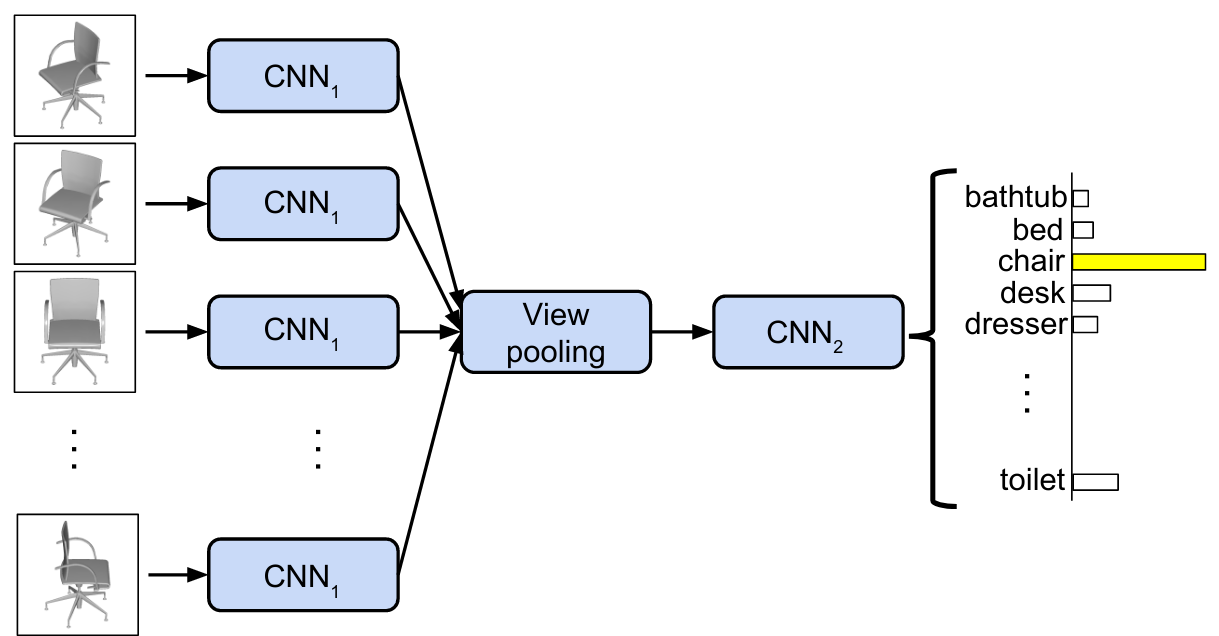
This approach was so successful, outperforming all contemporary approaches in both computational requirements and accuracy, that it served as the baseline to compare against for year to follow.
A similar idea was used in Multi-View 3D Object Detection Network for Autonomous Driving to not only classify, but also detect objects. Instead of using multiple rendered views, they made use of the LiDAR point cloud, which was projected into a front view (similar to a depth image one obtains from RGB-D cameras, but much sparser) and multiple Bird’s eye views, i.e. looking at the point cloud from above and slicing it into multiple “depth-planes” along its height.
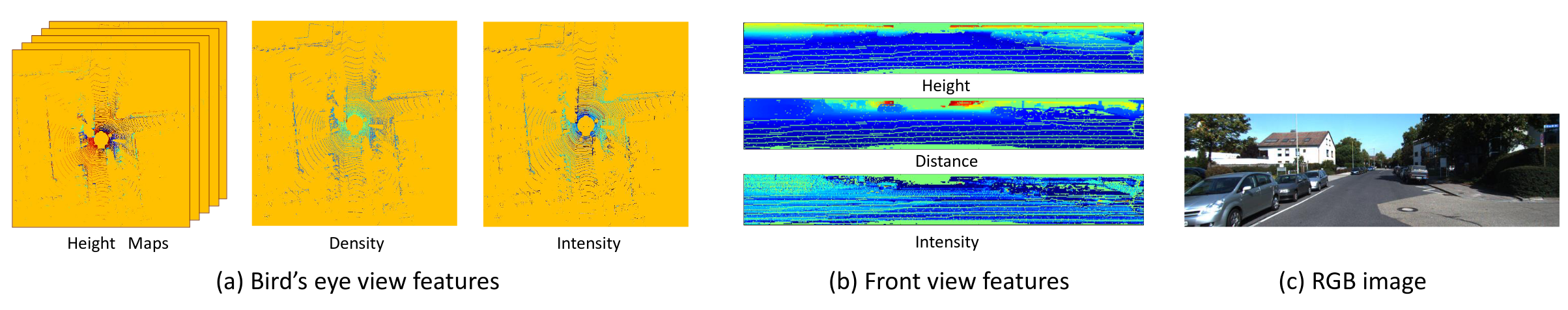
Because the obtained representation are quite different from one another (e.g. RGB images and point cloud bird’s eye view images), the resulting model architecture is quite convoluted2 (as is common in object detection) but at least conceptually it’s a simple approach and it worked quite well.
The geometric primitives approach
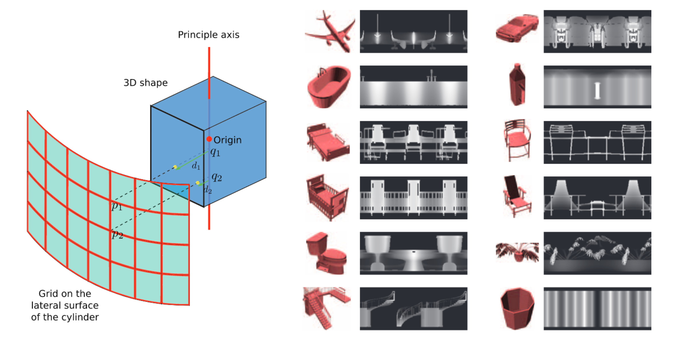
While not an officially recognised category, projecting 3D objects onto geometric primitives is nonetheless quite common. In DeepPano: Deep Panoramic Representation for 3-D Shape Recognition, the authors projected each object onto a cylinder, placed around the objects’ principal axis. One can think about this as an extension to the multi-view approach, but with infinitely many views (at least around one axis).
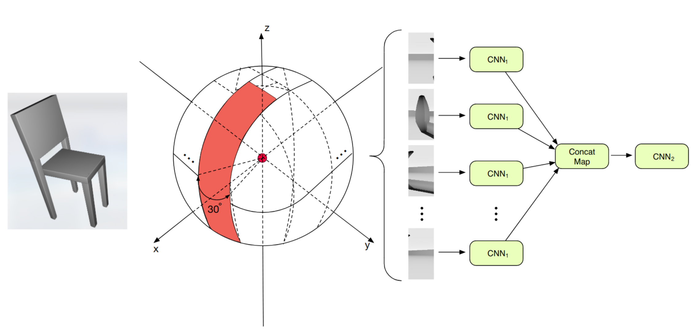
Now, you might wonder, if one can use object panoramas, why not use 360° views? And of course this is exactly what was done in 3D Object Classification via Spherical Projections. Once the object is projected onto the sphere, the authors cut it into stripes and fed those to a CNN. As you might notice from the right part of the image below, the model architecture is very similar to multi-view CNN we have seen before. This was one of the first works to outperform the classical multi-view approach, but the authors additionally showed, that using a pre-trained network can help to boost classification performance significantly.
Finally, in a similar approach as the previous one, the authors of Deep Learning 3D Shape Surfaces Using Geometry Images also made use of a spherical projections, but subsequently mapped the sphere onto a 2D plane, as shown below. This has the theoretical advantage, that less discontinuities are introduced compared to cutting the sphere into stripes, which can potentially make the task easier to learn for a CNN.
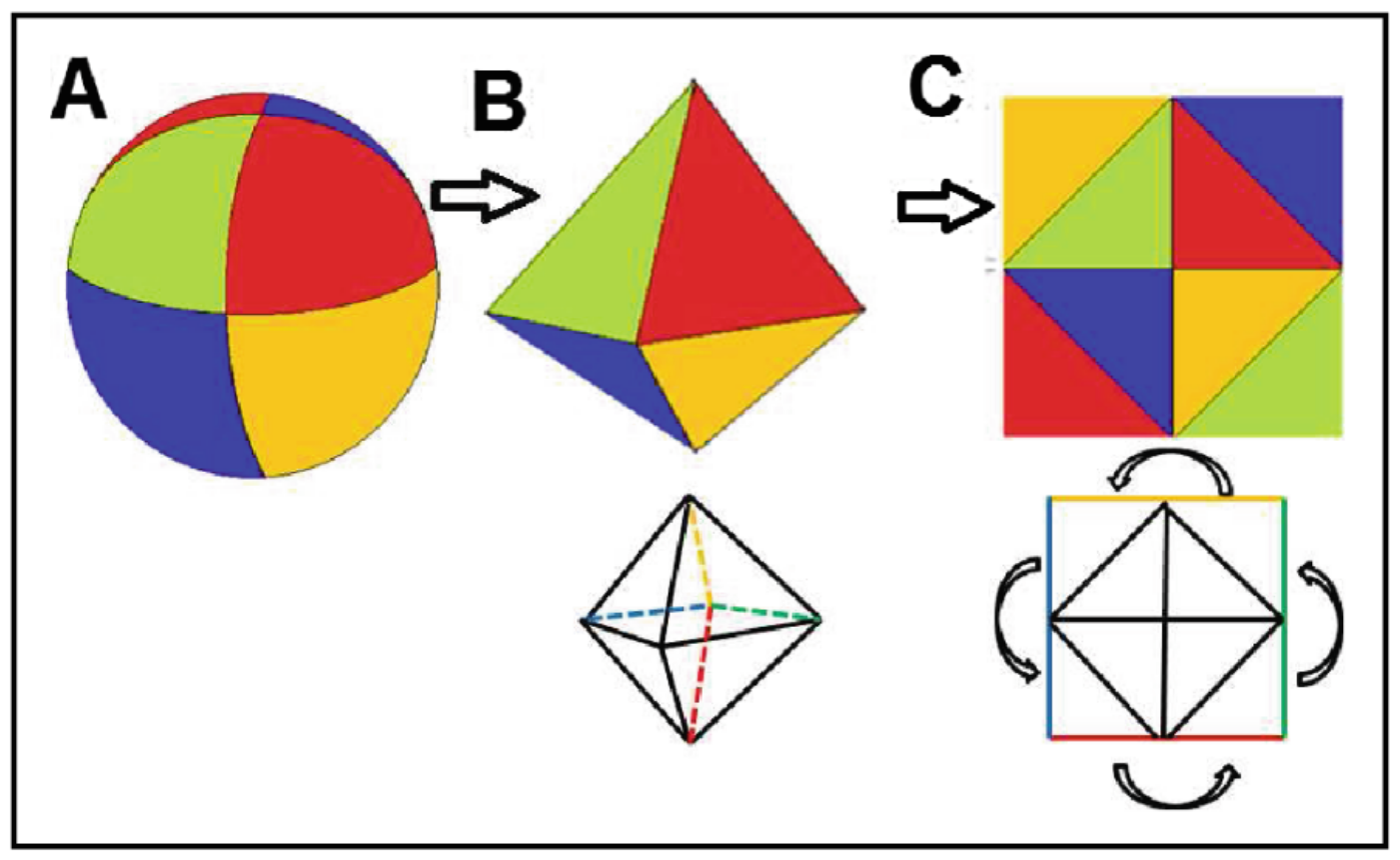
Due to the continuity of the representation, it can also be used to learn to classify non-rigid objects, i.e. objects that are soft and can deform. Unfortunately, the theoretical advantages of this work didn’t translate too well into increased performance.
Wrapping up
This final chapter concludes the series on the various ways to learn from three dimensional data. There might be more, but point clouds, voxel grids, graphs and meshes and projections are the four big ones I came across during my research. We will probably come back to 3D deep learning in the future on this blog, as I have chosen to pursue the topic for my PhD, but for the immediate future I have some other long overdue article ideas in the making. Stay tuned!